From CSBLwiki
Biomodel database
Running SBML
R-project
Matlab
M = getstoichmatrix(modelObj)
[M,objSpecies] = getstoichmatrix(modelObj)
[M,objSpecies,objReactions] = getstoichmatrix(modelObj)
Readings
- Books
- Math tutorials
- Metabolic Control Analysis (MCA)
Term project
2009 Fall
- 지난수업시간에 공지한것처럼 기말 프로젝트로 다음 세가지 옵션중 1개를 선택하여 12/18(금)까지 제출해 주십시오.
- Matlab을 이용한 SBML 읽기 및 모델링 - Biomodel database (http://www.ebi.ac.uk/biomodels-main/) 에서 테스트를 원하는 모델을 SBML형식으로 다운로드 받아서 Matlab에서 읽고, Default parameter로 시뮬레이션을 합니다 (제출해야할것 - 작동하는 Matlab 코드, 사용한 SBML화일) <=== 현재 the third party toolbox gives errors to handle BIOMODEL SBMLs. You may modify the SBML file (e.g. symbols)
- R package를 사용한 SBML읽기 - 현재 SBMLR library package가 불완전하여 모든 SBML을 성공적으로 읽지 못합니다. 따라서 KEGG에 있는 sde00010 pathway (glycolysis in Saccharophagus degradans)를 SBMLR이 읽을 수 있는 형태 (e.g. readSBMLR)로 변환하여 R 에서 읽습니다 (제출해야할것 - R 의 SBMLR이 읽을수 있는 sde00010 pathway 화일)
- Matlab이나 R을 사용하지 하는 경우, KEGG에 있는 sde00010 pathway의 전체 stoichiometric matrix(S)를 MS-Excel화일에 직접 작성합니다. 이때, row는 species, column은 reaction으로 합니다 (제출해야할것 - stoichiometric matrix를 포함한 MS-Excel화일)
- Reconstructing central carbon pathways in target organims
- Example using SBMLR
- Curto, R., Voit, E. O. and Cascante, M. Analysis of abnormalities in purine metabolism leading to gout and to neurological dysfunctions in man. Biochem.J. 329 (Pt 3), 477-487 (1998a).
- Curto, R., Voit, E. O., Sorribas, A. and Cascante, M. Validation and steady-state analysis of a power-law model of purine metabolism in man. Biochem.J. 324 (Pt 3), 761-775 (1997).
- Curto, R., Voit, E. O., Sorribas, A. and Cascante, M. Mathematical models of purine metabolism in man. Math.Biosci. 151, 1-49 (1998b)
## installing Bioconductor
source("http://bioconductor.org/biocLite.R")
biocLite() # install default packages
biocLite(c("KEGGgraph","SBMLR")) # install specified packages
## loading packages by 'library' function
library(KEGGgraph)
##
##---- The following example performs a perturbation in PRPP from 5 to 50 uM in Curto et al.
##
library(SBMLR)
library(odesolve)
curto=readSBML(file.path(system.file(package="SBMLR"), "models/curto.xml"))
summary(curto)
names(curto)
out1=simulate(curto,seq(-20,0,1))
curto$species$PRPP$ic=50
out2=simulate(curto,0:70)
outs=data.frame(rbind(out1,out2))
attach(outs)
par(mfrow=c(2,1))
plot(time,IMP,type="l")
plot(time,HX,type="l")
par(mfrow=c(1,1))
detach(outs)
# which should be the same plots as
curto=readSBMLR(file.path(system.file(package="SBMLR"), "models/curto.r"))
out1=simulate(curto,seq(-20,0,1))
curto$species$PRPP$ic=50
out2=simulate(curto,0:70)
outs=data.frame(rbind(out1,out2))
attach(outs)
par(mfrow=c(2,1))
plot(time,IMP,type="l")
plot(time,HX,type="l")
par(mfrow=c(1,1))
detach(outs)
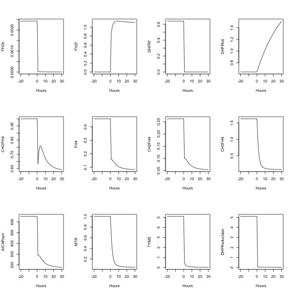
##---- The following example uses fderiv to generate Morrison's folate system response to
morr=readSBMLR(file.path(system.file(package="SBMLR"), "models/morrison.r"))
out1=simulate(morr,seq(-20,0,1))
morr$species$EMTX$ic=1
out2=simulate(morr,0:30)
outs=data.frame(rbind(out1,out2))
attach(outs)
pdf(file="output.pdf",paper="A4")
par(mfrow=c(3,4))
plot(time,FH2b,type="l",xlab="Hours")
plot(time,FH2f,type="l",xlab="Hours")
plot(time,DHFRf,type="l",xlab="Hours")
plot(time,DHFRtot,type="l",xlab="Hours")
plot(time,CHOFH4,type="l",xlab="Hours")
plot(time,FH4,type="l",xlab="Hours")
plot(time,CH2FH4,type="l",xlab="Hours")
plot(time,CH3FH4,type="l",xlab="Hours")
plot(time,AICARsyn,type="l",xlab="Hours")
plot(time,MTR,type="l",xlab="Hours")
plot(time,TYMS,type="l",xlab="Hours")
#plot(time,EMTX,type="l",xlab="Hours")
plot(time,DHFReductase,type="l",xlab="Hours")
dev.off()